Neuroimaging
From ACL@NCU
Overall Concept
Design Issues
In practice, real fMRI noise means that two or three-block designs may have blocks that are too long to be optimal. Skudlarksi et. al (see DesignPapers), using real fMRI noise and simulated signal, recommend about 18 seconds for complex cognitive tasks where the response time (and time of initial hemodynamic response onset) is somewhat uncertain (on the order of a couple seconds). For simple sensory or motor tasks with less uncertainty in that response, shorter blocks (12 seconds or so) may be appropriate. Of course, you should always take into account the psychological load of your blocks; with especially long blocks, the qualitative experience may change due to fatigue or other factors, which would influence your results.
Bledowski et al. (2006, HrfPapers), using empirically derived estimates of the HRF, mathematically derive a 7-sec-on, 7-sec-off block pattern as being optimal for maximizing BOLD response, suggesting it's a bit like a "swing" - pushing for the first half, then letting go, maximizes your amplitude.
Statistics
(Excerpt from Mindhive) "The FIR model is a modification of the standard GLM which is designed precisely to deconvolve different conditions' peristimulus timecourses from each other. The main modification from the standard GLM is that instead of having one column for each effect, you have as many columns as you want timepoints in your peristimulus timecourse. If you want a 30-second timecourse and have a 3-second TR, you'd have 10 columns for each condition. Instead of having a single model of activity over time in one column, such as a boxcar convolved with a canonical HRF, or a canonical HRF by itself, each column represents one timepoint in the peristimulus timecourse. So the first column for each condition codes for the onset of each trial; it has a single 1 at each TR that condition has a trial onset, and zeros elsewhere. The second column for each condition codes for the onset + 1 point for each trial; it has a single 1 at each TR that's right after a trial onset, and zeros elsewhere. The third column codes in the same way for the onset + 2 timepoint for each trial; it has a single 1 at each TR that's two after a trial onset, and zeros elsewhere. Each column is filled out appropriately in the same fashion."
- Parametric modulation (from mindhive)
How does parametric modulation work? When would I use it?
As described above, there are all kind of modifications the researcher can make to her design matrix once she's described the basics of when her conditions are happening. One important one is parametric modulation, which can be used in a case where an experimental condition is not just ON or OFF, but can happen at a variety of levels during the experiment. An example might be an n-back memory task, where on each trial the subject is asked to remember what letter happened n trials before, where n is varied from trial to trial. One hypothesis the research might have is that activity in the brain varies as a function of n - remembering back 3 trials is harder than remembering 1, so you might expect activity on a 3-back trial to be higher than on a 1-back. In this case, a parametric modulation of the design matrix would be perfect.
Generally, a parametric modulation is useful if you have some numerical value for each trial that you'd like to model. This contrasts with having a numerical value to model at each timepoint, which would be a time for a user-specified regressor (see below). In the parametric case, the user specifies onset times for the condition, and then specifies a parameter value for each trial in the condition - if there are 10 n-back trials, the user specifies 10 parameter values. The design matrix then modulates the activity in that column for each trial by some function of the parameter - linear, exponential, polynomial, etc. - set by the user. If the hypothesis is correct, that modulated column will fit the activity significantly better than an unmodulated effect. In SPM (and possibly others), the program splits the effect into two columns - an unmodulated effect and a parametric column - so that the researcher can separately estimate the effect of the condition itself and of the parametric modulation of that effect. This would be a way of separating out, in the example, the effect of doing any kind of retrieval from the load effect of varying the parameter.
- Reaction Time modeling (from mindhive)
What's the best way to include reaction times in my model? If you have events for which participants' response times vary widely (or even a little), your model will be improved by accounting for this variation (rather than assuming all events take identical time, as in the normal model). A common way of including reaction times is to use a parametric modulator, with the reaction time for each trial included as the parameter. In the most common way of doing this, the height of the HRF will be thus modulated by the reaction time. Grinband et al. (HBM06) showed this method actually doesn't work as well as a different kind of parametric regression - in which each event is modeled as an epoch (i.e., a boxcar) of variable duration, convolved with a standard HRF.
In other words, rather than assuming that neural events all take the same time, and the HRF they're convolved by varies in height with reaction time (not very plausible, or, it turns out, efficient), the best way is to assume the underlying neural events vary in reaction time, and convolve those boxcars (rather than "stick functions") with the same HRF.
In either case, as with most parametric modulation, the regressor including reaction time effects can be separate from the "trial regressor" that models the reaction-time-invariant effect of the trial. This corresponds to having one column in the design matrix for the condition itself (which doesn't have any reaction time effects) and a second, parametrically modulated one, which includes reaction times. If your goal is merely to get the best model possible, these don't need to be separated (only the second of the two, which includes RTs, could go in the model), but this will not allow you to separate the effect of "just being in the trial" from neural activations that vary with reaction time. To separate those effects, you need separate design matrix columns to model them. That choice depends on how interested you are in the reaction-time effect itself.
Smoothing
(Excerpt from Mindhive) The first point at which it's obvious to smooth is as the last spatial preprocessing step for your raw images; smoothing before then will only reduce the accuracy of the earlier preprocessing (normalization, realignment, etc.) - those programs that need smooth images do their own smoothing in memory as part of the calculation, and don't save the smoothed versions. One could also avoid smoothing the raw images entirely and instead smooth the beta and/or contrast images. In terms of efficiency, there's not much difference - smoothing even hundreds of raw images is a very fast process. So the question is one of performance - which is better for your sensitivity?
Skudlarski et. al (SmoothingPapers) evaluated this for single-subject data and found almost no difference between the two methods. They did find that multifiltering (see below) had greater benefits when the smoothing was done on the raw images as opposed to the statistical maps. Certainly if you want to use p-values corrected with Gaussian field theory (a la SPM), you need to smooth before estimating your results. It's a bit of a toss-up, though...
AFNI know-how
Preprocessing
- Data import
- use to3d or dimon to convert raw images into AFNI BRIK format
- to3d_anat.py, to3d_func.py
- Data file organizations
- creating group list
- getid.py
- looking for the sequential order ID one or more subjects
- lookup_subj.py
- lookup_subj_many.py
- Deoblique
- N.B.: EPI time series data should be time shifted with 3dTshift before rotating the volumes to a cardinal direction
3dWarp -deoblique
Individual level GLM
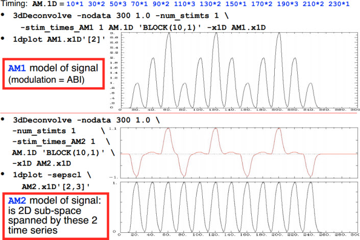
- -stim_times_AM1 and -stim_times_AM2[1]
Group analysis[2]
- Average group T
Copy 3D+tlrc.BRIK & .HEAD into your "average" directory
3dmerge -doall 3d*+tlrc*
(where "3d*+tlrc* is using enough wild cards to get all the 3D anatomy files you want to average)
The output name is mrg+tlrc.BRIK and mrg+tlrc.HEAD by default, but you can use the -prefix flag to specify an output prefix (other than mrg) that you prefer.
Program 3dMVM in the AFNI suite is a program that runs FMRI group analysis with a multivariate modeling approach.
Gang Chen: "3dMEMA is developed in R with a mixed-effects meta analysis (MEMA) approach. It effectively takes advantage of estimate precision from each subject, and assigns each subject's contribution in the final result based on weighting instead of equal treatment. More specifically, a more precise beta estimate (meaning higher t-statistic) from a subject will have more say in the group effect; conversely, a less reliable beta estimate (i.e., lower t-statistic) from a subject will be discounted in the MEMA model. Such strategy can be surprisingly tolerant of and robust against some types of outliers compared to the conventional group analysis method."
Multiple comparison
- What smoothness parameters should one use for 3dClustSim for results of group analysis?
1. Nick: "You could use a single subject but it's better to take the average across subjects for a more reliable estimate.
That said, in my experience smoothness estimates don't vary that much across subjects if in the same study and everything else is equal (like scanning and preprocessing parameters). "[3]
2. Regarding blur estimates, expect to get estimates per subject and then average those together. You do not want the errts time series averaged down to zero before running 3dFWHMx, as that might play havoc with the estimates (the data might look VERY blurry, I don't know). But I would not expect averaging the errts datasets to increase the reliability of the blur estimation. Averaging over the errts and then over subjects is already (hopefully) generating a very robust estimate. (Rick Reynolds)[4]
Region-of-Interest (ROI)
- Creating a half hemisphere mask
#left hemisphere selected
3dcalc -a mask_group+tlrc. -expr 'step(x-0)' -prefix test

#intersection with brain mask, and save in rh_mask+tlrc
3dcalc -a mask_group+tlrc. -b test+tlrc -expr 'step(a*b)' \
       -prefix rh_mask
- Convert a multi-cluster mask to a union mask (each ROI with the same value)
3dcalc -a Clust_N_Control_p005_mask+tlrc -expr 'notzero(a)' -prefix Clust_N_Control_p005_maskp
Connectivity Analysis
DWI Data Analysis
- AFNI DTI tutorial: [ http://openwetware.org/wiki/Beauchamp:ProcessDiffTensImgData]
Misc.
- Converting a single t-value to z-value
ccalc -expr 'fitt_t2z(t, n)'
t: tvalue
n: degrees of freedom
- Converting t-value sub-brick to z-value sub-brick
3dcalc -a dset+tlrc[<t-map_id>] \
  -expr 'fitt_t2z(3, 10)' -prefix dset2
- listing all subbriks in a BRIK file and add numerical index
3dinfo -label <BRIK filename> | sed 's/|/\n/g' | nl -v0
- Segmentation (not recommended for quantitative use)
3dSeg 	-anat <anatfile> -mask AUTO \
	-classes 'CSF ; GM ; WM' -bias_classes 'GM ; WM' \
      	-bias_fwhm 25 -mixfrac UNI -main_N 5 \
      	-blur_meth BFT -prefix <output file>
- Extracting grey matter mask from segmented brain
3dcalc -a Classes+tlrc'<GM>' -expr 'step(a)' \
       -prefix TT_icbm452_GMseg
- resample the mask to a coarse resolution
3dresample -dxyz 3 3 3 -rmode 'Cu'        \
             -inset TT_icbm452_GMseg+tlrc \
             -prefix TT_icbm_GMseg3mm
- Combining multiple mask files under subdirectories
3dmask_tool -input `find . -name "mask_anat*.HEAD" ` \
              -prefix mask_overlap.7 -frac 0.7
- Create partial union mask for a group of anatomical masks
#partial union mask
3dmask_tool -frac 0.3 -input *_GMseg+tlrc.HEAD \
            -prefix punion_0.3.mask
- Look-up dicom raw data header (ID creation time in this case)
dicom_hdr <filename> | grep 'ID Instance Creation Time'
- Use 3dTstat to carry out numerical computations on 1D files[5]
3dTstat -mean -stdev -prefix - fred.1D'[3..8]{5..9}'\' > tjed.1D
1dtranspose fred.1D | 1dplot -stdin
- apply 3drefit on multiple files
#usage run_refitclustsim '<prefix>'
#the single quote is necessary to enlist multiple file names
#in the argument of the command script
set statfn =  (`ls $argv[1]`)
- compute algebra on multiple columns from a file
#contents of a file (tmp)
 22.7758 -23.44 -3.5621
 22.7758 -27.44 -5.5621
 22.7758 -25.44 -5.5621
 22.7758 -23.44 -5.5621
.............
 22.7758 -27.44 -7.5621
 22.7758 -25.44 -7.5621
 22.7758 -23.44 -7.5621
 22.7758 -27.44 -9.5621

#Use 3dTstat to compute column parameters
#Transpose (\') and *.1D files is required
3dTstat  -overwrite -mean \
	-prefix stdout: tmp.1D\'


<\pre>

= BrainVoyager QX know-how =

== Preprocessing ==
== Individual level GLM ==
== Group analysis ==
*Created individual vmps[http://support.brainvoyager.com/functional-analysis-statistics/36-glm-modelling-multi-study/245-how-to-analyze-multiple-vmps-using-the-combine-vmp-option.html]
*Paired t-test on vmps[http://support.brainvoyager.com/documents/DWI/PAIREDt.pdf]

== Multiple comparison ==
*Cluster threshold estimation (CTE)
**Forming valid mask[http://www.brainvoyager.com/ubb/Forum11/HTML/000101.html]
**Masking and cluster thresholding[http://www.brainvoyager.com/ubb/Forum11/HTML/000047.html]
**CTE in BVQX vs. other softwares (AFNI, SPM)[http://www.brainvoyager.com/ubb/Forum4/HTML/000814.html]
**[[CTE_mask|Solution to "Mask Not Valid!!" problem in CTE]]

== Region-of-Interest (ROI) ==

=FreeSurfurer tutorials=
*view data
<pre>
tkmedit sub001 brain.finalsurfs.mgz -aux T1.mgz -surfs -aseg
- syntax
- sub001: Subject ID
- brain.finalsurfs.mgz: skull-stripped volume primarily used for troubleshooting (found in $SUBJECTS_DIR/good_output/mri).
- aux T1.mgz : pre-skull-stripped volume loaded as 2nd volume (in $SUBJECTS_DIR/good_output/mri)
- surfs : loads all surfaces (orig, white, and pial, for left and right hemispheres)
- aseg : loads automatic volume segmentation called aseg.mgz
Online Database
openfmri
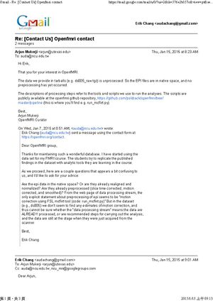
This is a database maintained by Russ Poldrack's group. It provides functional and behavioral data for a full replication of published reports. The data came in .

MVPA concepts and tools
concepts
- Neural Computation: Population Coding of High-Level Representations
- Machine learning classifiers and fMRI: a tutorial overview
- The Elements of Statistical Learning: Data Mining, Inference, and Prediction
tools
| Toolbox | Platform | Author |
| Princeton MVPA toolbox | MATLAB | |
| Decoding Toolbox | MATLAB | Martin Hebart |
| PyMVPA | python | |
| scikit learn | python |
DTI
TORTOISE
% Program caused arithmetic error: Floating underflow
% Program caused arithmetic error: Floating illegal operand

This is normal and can happen in both DIFF_PREP and DIFF_CALC.
It is a preference of IDL to keep these statments in.
It will not affect the results or functionality of the software in any way.

